Original Link: https://www.anandtech.com/show/6808/westmereep-to-sandy-bridgeep-the-scientist-potential-upgrade
Westmere-EP to Sandy Bridge-EP: The Scientist Potential Upgrade
by Ian Cutress on March 4, 2013 9:30 AM EST- Posted in
- CPUs
- Xeon
- Westmere-EP
- Sandy Bridge-EP
Earlier this year I wrote a review of a dual processor Sandy Bridge-EP system from the point of view of the non-CS trained coder in a research group, and whether the limited knowledge of advanced processor commands (beyond basic C++ with OpenMP) was a hindrance to dual processor systems on some simple grid solvers/Brownian motion simulation. As part of the feedback to the review, I was asked by several readers using the older Westmere-EP platform doing similar types of calculations if it was worth pushing their research budget for a move from Westmere-EP to high-end Sandy Bridge-E, and whether the jump in cores/IPC would cost effective in those simulation scenarios. Thankfully Gigabyte was on hand to supply their GA-7TESM DP socket 1366 Xeon board and a pair of X5690s in order to run the comparison.
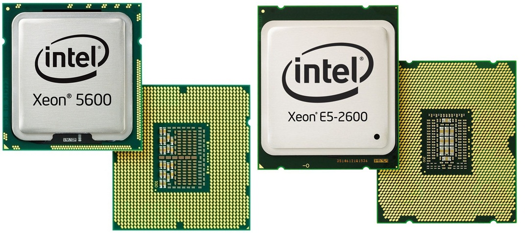
Comparing Westmere-EP to Sandy Bridge-EP
Johan’s words say it best, from his article on the E5-2600 in March 2012:
Compared to its predecessor, the Xeon X5600, the Xeon E5-2600 offers a number of improvements:
A completely improved core, as described here in Anand's article. For example, the µop cache lowers the pressure on the decoding stages and lowers power consumption, killing two birds with one stone. Other core improvements include an improved branch prediction unit and a more efficient Out-of-Order backend with larger buffers.
A vastly improved Turbo 2.0. The CPU can briefly go beyond the TDP limits, and when returning to the TDP limit, the CPU can sustain higher "steady-state" clockspeed. According to Intel, enabling turbo allows the Xeon E5 to perform 14% better in the SAP S&D 2 tier test. This compares well with the Turbo inside the Xeon 5600 which could only boost performance by 4% in the SAP benchmark.
Support for AVX Instructions combined with doubling the load bandwidth should allow the Xeon to double the peak floating point performance compared to the Xeon "Westmere" 5600.
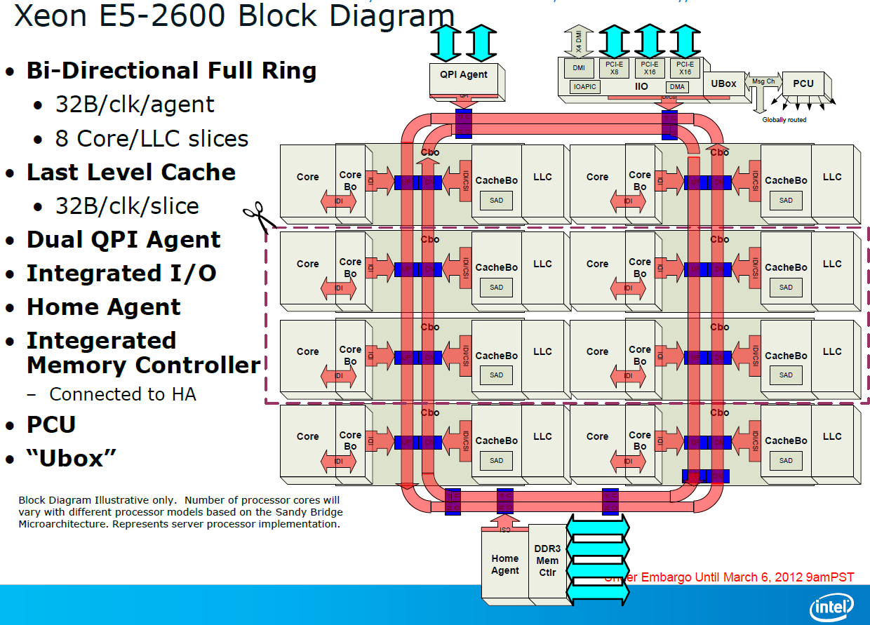
A bi-directional 32 byte ring interconnect that connects the 8 cores, the L3-cache, the QPI agent and the integrated memory controller. The ring replaces the individual wires from each core to the L3-cache. One of the advantages is that the wiring to the L3-cache can be simplified and it is easier to make the bandwidth scale with the number of cores. The disadvantage is that the latency is variable: it depends on how many hops a certain piece of data inside the L3-cache must cross before ends up at the right core.
A faster QPI: revision 1.1, which delivers up to 8 GT/s instead of 6.4 GT/s (Westmere).
Lower latency to PCI-e devices. Intel integrated a PCIe 3.0 I/O subsystem inside the die which sits on the same bi-directional 32 bit ring as the cores. PCIe 3.0 runs at 8 GT/s (PCIe 2.0: 5 GT/s), but the encoding has less overhead. As a result, PCIe 3.0 can deliver up to 1 GB full duplex per second per lane, which is twice as much as PCIe 2.0.
Removing the I/O lowered PCIe latency by 25% on average according to Intel. If you only access the local memory, Intel measured 32% lower read latency.
The access latency to PCIe I/O devices is not only significantly lower, but Intel's Data Direct I/O Technology allows the PCIe NICs to read and write directly to the L3-cache instead of to the main memory. In extremely bandwidth constrained situations (using 4 Infiniband controllers or similar), this lowers power consumption and reduces latency by another 18%, which is a boon to HPC users with 10G Ethernet or Infiniband NICs.
The new Xeon also supports faster DDR3-1600, up to 2 DIMMs per channel that can run at 1600 MHz.
Ian’s Analysis
In my line of computational chemistry, several E5-2600 characteristics would be very important to throughput:
- The improved core and µop cache should boost IPC through the roof with calculations that can take advantage, especially advanced trigonometric functions.
- The increase in L3 cache would reduce stress on jumps out to main memory for values, although the improved memory bandwidth would also help in this regard.
- More cores are always welcome – Turbo 2.0 would help with pre-release code testing, which often occurs in debug / single thread mode.
- An increase of memory limits would help various simulation scenarios, as well as aid having VMs of different environments.
- The move up to PCIe 3.0 helps any GPGPU simulation that requires lots of memory transfers back and forth across the bus (matrix solving), as long as the GPU supports PCIe 3.0 (K10, K20X, FirePro, not Xeon Phi which uses PCIe 2.0).
We all know the E5-2600 series is faster (one reader in response to the previous review had seen slowdown in parts of his code on E5-2600), but the question is always around “how much?”.
On paper, Johan’s article showed us the specifications side by side (along with Opteron counterparts):
|
Xeon E5-2600 Sandy Bridge-EP |
Opteron 6200 Interlagos |
Opteron 6100 Magny-Cours |
Xeon 5600 Westmere |
|
|
Cores/Threads Modules/Threads |
8/16 | 12/12 | 6/12 | |
| 8/16 | ||||
| L1 Instruction |
8x 32KB 4-way |
8x 64KB 2-way |
12x 64KB 2-way |
6x 32KB 4-way |
| L1 Data |
8x 32KB 8-way |
16x 16KB 4-way |
12x 64KB 2-way |
6x 32KB 8-way |
| L2 Cache | 8x 256 KB | 4x 2MB | 12x 512KB | 6x 256KB |
| L3 Cache | 20 MB | 2x 8MB | 2x 6MB | 12 MB |
|
Mem Bandwidth (Per Socket) |
51.2 GB/s | 51.2 GB/s | 42.6 GB/s | 32 GB/s |
| IMC Clock Speed | On Die | 2 GHz | 1.8 GHz | 2 GHz |
| Interconnect |
2x QPI 2.0 8 GT/s |
4x HT 3.1 6.4 GT/s |
4x HT 3.1 6.4 GT/s |
2x QPI 4.8-6.4 GT/s |
| Transistors | 2.26 B | 2x 1.2 B | 2x 0.9 B | 1.17 B |
| Die Size mm2 | 416 | 2x 315 | 2x 346 | 248 |
As well as the subsequent pricing difference:
| Intel vs. Intel 2-socket SKU Comparison | |||||||||
|
Xeon 5600 |
Cores/ Threads |
TDP |
Clock (GHz) |
Price |
Xeon E-5 |
Cores/ Threads |
TDP |
Clock (GHz) |
Price |
| High Performance | High Performance | ||||||||
| 2690 | 8/16 | 135W | 2.9/3.3/3.8 | $2057 | |||||
| X5690 | 6/12 | 130W | 3.46/3.6/3.73 | $1663 | 2680 | 8/16 | 130W | 2.7/3.1/3.5 | $1723 |
| 2670 | 8/16 | 115W | 2.6/3/3.3 | $1552 | |||||
| 2665 | 8/16 | 115W | 2.4/2.8/3.1 | $1440 | |||||
| X5675 | 6/12 | 95W | 3.06/3.33/3.46 | $1440 | |||||
| X5660 | 6/12 | 95W | 2.8/3.06/3.2 | $1219 | 2660 | 8/16 | 95W | 2.2/2.6/3.0 | $1329 |
| X5650 | 6/12 | 95W | 2.66/2.93/3.06 | $996 | 2650 | 8/16 | 95W | 2/2.4/2.8 | $1107 |
| Midrange | Midrange | ||||||||
| E5649 | 6/12 | 80W | 2.53/2.66/2.8 | $774 | 2640 | 6/12 | 95W | 2.5/2.5/3 | $885 |
| 2630 | 6/12 | 95W | 2.3/2.3/2.8 | $612 | |||||
| E5645 | 6/12 | 80W | 2.4/2.53/2.66 | $551 | |||||
| 2620 | 6/12 | 95W | 2/2/2.5 | $406 | |||||
| E5620 | 4/8 | 80W | 2.4/2.53/2.66 | $387 | |||||
| High clock / budget | High clock / budget | ||||||||
| X5647 | 4/8 | 130W | 2.93/3.06/3.2 | $774 | 2643 | 4/8 | 130W | 3.3/3.3/3.5 | $885 |
| E5630 | 4/8 | 80W | 2.53/2.66/2.8 | $551 | |||||
| E5607 | 4/4 | 80W | 2.26 | $276 | 2609 | 4/4 | 80W | 2.4 | $294 |
| Power Optimized | Power Optimized | ||||||||
| L5640 | 6/12 | 60W | 2.26/2.4/2.66 | $996 | 2650L | 8/16 | 70W | 1.8/2/2.3 | $1107 |
| 5630 | 4/8 | 40W | 2.13/2.26/2.4 | $551 | 2630L | 8/16 | 60W | 2/2/2.5 | $662 |
In my experience, workstations for research are often prebuilt, so if the system builder makes a 10% markup, this would extrapolate the prices even more. For the processors we are focusing on today, the boxed version of the X5690 sits at $1666 each and the E5-2690 is $2061 – about a 25% price difference moving up to the E5-2690. However as a system the price difference may be slightly more, when we include memory and power supplies into the mix – even more if you want to expand the functionality for new interfaces. When dealing with a personal machine, a user can often recoup the cost by selling on the old hardware, making the cost more palatable – the research group cannot do the same, and more often than not the old hardware gets passed down to experimentalists, or sits in the corner when extra CPU power is needed. That makes the price an absolute cost, rather than an upgrade difference.
Whenever I get told that a component is too expensive (a lot of users are currently berating the price of NVIDIA’s GTX Titan, for example), my response is often this:
- Look at what you are currently using, and the performance increase that the better part would give
- If time is money, calculate how much time you would save using the newer component. Convert that into a cost benefit analysis (i.e. completing a contract in 6 months rather than 7 months) as more computation can be processed.
- If the cost can be recouped over 12 months, the purchase is probably justified (depending on who finances what) and will allow you to consider another upgrade in 12 months.
It is quite rare to be in a situation where the computational time is the limiting factor in a project, although I do acknowledge that when dealing with long simulations or calculations it can be. But if you can finish analyzing results in 4 hours rather than 6, if there is an error, it can be fixed and re-run in a shorter time. Essentially the more you require computational throughput for a project, the better the cost analysis usually is.
With all this said, the proof is always going to be in the numbers – I would suggest that for each situation our readers face, to weigh up the computational aspects of their work. In research, I spent more time organizing mathematics and coding than simulating, though when simulating some of them would take a week on a GTX 480 GPU, and I would run several batches at once. If Titan was around then and could save 40% of that time, I would have plugged my research supervisor for one in an instant. Similar arguments would have been made on the non-GPU side of the research, as often we would use each other’s 16 thread machines to get stuff done (and then repeat it if there was a coding error).
Test Setup
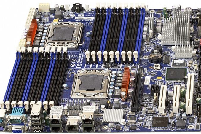
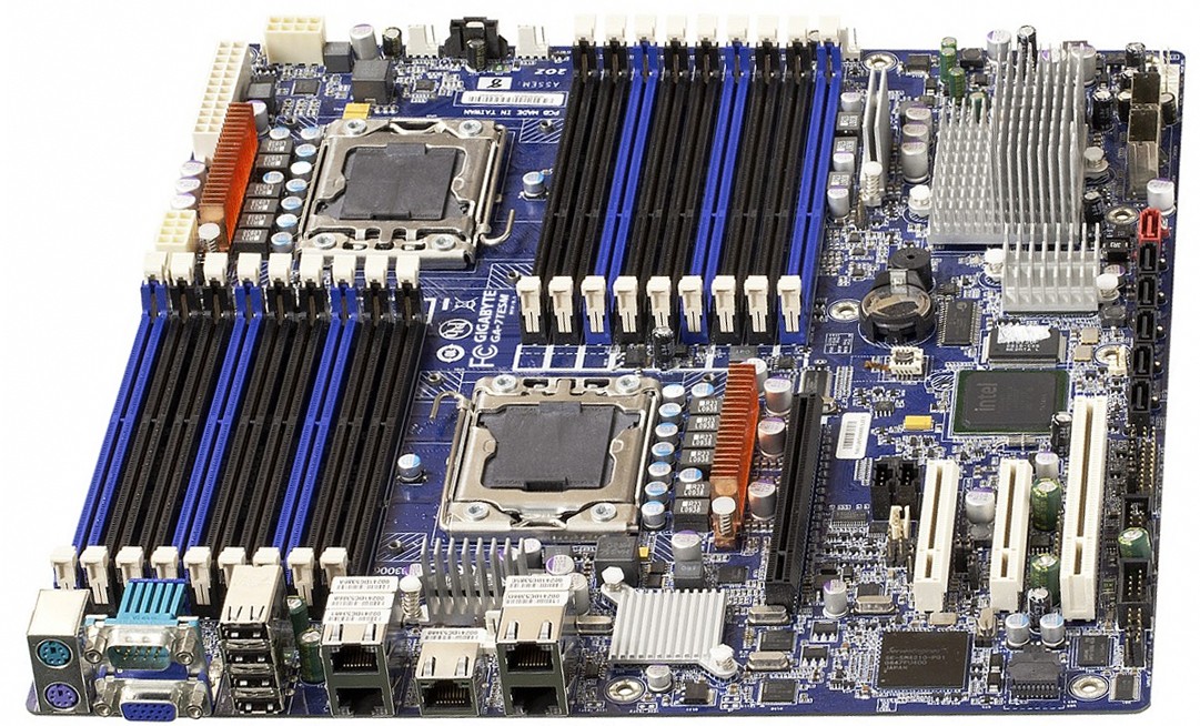
Alongside the X5690 CPUs we are using for this review, the Gigabyte server team was at hand to offer one of their dual processor 1366 server motherboards – the GA-7TESM. The 7TESM was released back in September 2011, featuring support for 55xx/56xx Xeons and up to 18 DIMMs of registered or unbuffered DDR3 memory – for up to 288GB at 1333 MHz with Netlist Hypercloud modules. Alongside four Intel GbE network ports (82576EB + 2x 82574L) and a management port, we get six SATA 3 Gbps ports from the chipset and 8 SAS 6 Gbps ports from an LSI SAS2008 chip (via SFF-8087), both supporting RAID 0/1/5/10. Onboard video comes from a Matrox 200e, and the system provides a PCIe 2.0 x16, an x8, an x4, and a PCI slot. Many thanks to Gigabyte for making the review possible!
Many thanks also to...
We must thank the following companies for kindly providing hardware for our test bed:
Thank you to OCZ for providing us with the 1250W Gold Power Supply and SATA SSD.
Thank you to Kingston for providing us with the ECC Memory.
| Test Setup | |
| Processor |
2x Intel Xeon X5690 6 Cores, 12 Threads 3.47 GHz (3.73 GHz Turbo) each |
| Motherboards | Gigabyte GA-7TESM |
| Cooling | Intel Thermal Solution STS100C |
| Power Supply | OCZ 1250W Gold ZX Series |
| Memory | Kingston 1600 C11 ECC 8x4GB Kit |
| Memory Settings | 1333 C9 |
| Hard Drive | Kingston 120GB HyperX |
| Optical Drive | LG GH22NS50 |
| Case | Open Test Bed |
| Operating System | Windows 7 64-bit |
As per the last test with E5 2600 CPUs, we are using Windows 7 64 bit. The reason behind this is simple – in the research environment I was in, we never updated operating systems beyond security updates. IT staff wanted everyone in the building to use an approved OS image, of which there was only Windows XP, if anyone wanted network access. For this review I got in contact with a colleague to see if this is still the case, and it is – Windows XP 32-bit across the whole department at the university.
Power Consumption
Power consumption was tested on the system as a whole with a wall meter connected to the OCZ 1250W power supply, while in a single 7970 GPU configuration. This power supply is Gold rated, and as I am in the UK on a 230-240 V supply, leads to ~75% efficiency > 50W, and 90%+ efficiency at 250W, which is suitable for both idle and multi-GPU loading. This method of power reading allows us to compare the power management of the UEFI and the board to supply components with power under load, and includes typical PSU losses due to efficiency. These are the real world values that consumers may expect from a typical system (minus the monitor) using this motherboard.
While this method for power measurement may not be ideal, and you feel these numbers are not representative due to the high wattage power supply being used (we use the same PSU to remain consistent over a series of reviews, and the fact that some boards on our test bed get tested with three or four high powered GPUs), the important point to take away is the relationship between the numbers. These boards are all under the same conditions, and thus the differences between them should be easy to spot.
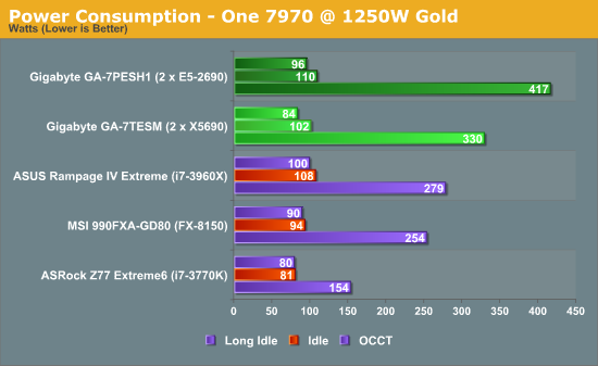
For the workstation theorist in a research group, power consumption is often the last thing on their minds – as long as the system computes in a decent time, everything is golden. In a commercial situation where the code works and throughput is everything, then power does matter. The Sandy Bridge-EP system used 26.3% more power during CPU load than our Westmere-EP system did, in line with the pricing of the CPU itself.
DPC Latency
Deferred Procedure Call latency is a way in which Windows handles interrupt servicing. In order to wait for a processor to acknowledge the request, the system will queue all interrupt requests by priority. Critical interrupts will be handled as soon as possible, whereas lesser priority requests, such as audio, will be further down the line. So if the audio device requires data, it will have to wait until the request is processed before the buffer is filled. If the device drivers of higher priority components in a system are poorly implemented, this can cause delays in request scheduling and process time, resulting in an empty audio buffer – this leads to characteristic audible pauses, pops and clicks. Having a bigger buffer and correctly implemented system drivers obviously helps in this regard. The DPC latency checker measures how much time is processing DPCs from driver invocation – the lower the value will result in better audio transfer at smaller buffer sizes. Results are measured in microseconds and taken as the peak latency while cycling through a series of short HD videos - under 500 microseconds usually gets the green light, but the lower the better.
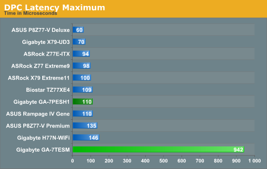
For whatever reason the DPC Latency on the X5690 system is bad. This is more indicative of the motherboard than the CPU performance, which should easily handle DPC requests. It is highly doubtful that time sensitive work would be carried out on a system like this, but any non-Xeon product would be able to outperform our setup.
Grid Solvers
For any theoretical evaluation of physical events, we mathematically track a volume and monitor the evolution of the properties within that volume (speed, temperature, concentration). How a property changes over time is defined by the equations of the system, often describing the rate of change of energy transfer, motion, or another property over time.
The volume itself is divided into smaller sections or ‘nodes’, which contain the values of the properties of the system at that point. The volume can be split a variety of different ways – regularly by squares (finite difference), irregularly by squares (finite difference with variable distance modifiers), irregularly by triangles (finite element) to name three, although many different methods exist. More often than not the system has a point of action where stuff is happening (heat transfer at a surface or a surface bound reaction), meaning that some areas of the system are more important than others and the grid solver should focus on those areas (benefits against regular finite difference). This usually comes at the expense of increased computational difficulty and irregular memory accesses, but affords faster simulation time having to calculate 1000 variable distance points rather than 1 million (as an example of a 106 simulation volume). Another point to note is that if the system is symmetrical about an axis (or the center), the simulation and grid chosen is often reduced by a dimension to improve simulation throughput (as O(n) < O(n2) < O(n3)).
Boundary conditions can also affect the simulation – because the volume being simulated is finite with edges, the action at those edges has to be determined. The volume may be one unit of a whole, making the boundary a repeating boundary (entering one side comes out the other), a reflecting boundary (rate of change at the boundary is zero), a sink (boundary is constantly 0), an input (boundary is constantly 1) or a reactive zone (rate of change is defined by kinetics or another property) – again, there are many more boundary conditions depending on the simulation at hand. However as the boundary conditions have to be treated differently, this can cause extended memory reads, additional calculations at various points, or fewer calculations by virtue of constant values.
A final point to make is dealing with simulations involving time. For the scenarios I simulated in research, time could either be dealt with as a pushing structure (every node in the next time step is based on the surrounding nodes ‘pushing‘ the values of the previous time step) or pulling structure (each calculation of the next time step requires pulling a matrix of values from the previous time step), also known as explicit and implicit respectively. By their nature, explicit simulations are embarrassingly parallel but have restricted conditions based on time step and node size – implicit simulations are only slightly parallel, require larger memory jumps but have several fewer restrictions that allow more to be simulated in less time. Deciding between these two methods is often one of the first decisions when it comes to the sorts of simulation I will be testing.
All of the simulations used in this article were described in our previous GA-7PESH1 review in terms of both mathematics and code. For the sake of brevity, please refer back to that article for more information.
Explicit Finite Difference
For any grid of regular nodes, the simplest way to calculate the next time step is to use the values of those around it. This makes for easy mathematics and parallel simulation, as each node calculated is only dependent on the previous time step, not the nodes around it on the current calculated time step. By choosing a regular grid, we reduce the levels of memory access required for irregular grids. We test both 2D and 3D explicit finite difference simulations with 2n nodes in each dimension, using OpenMP as the threading operator in single precision. The grid is isotropic and the boundary conditions are sinks.
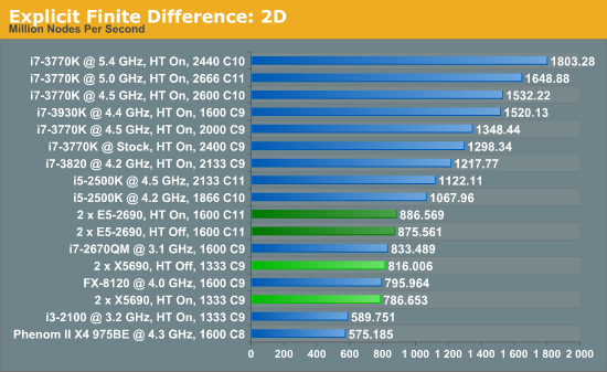
The 6-core X5690s in this situation definitely perform lower than the 8-core E5-2690s, although with the X5690s it pays to have HyperThreading turned off or face 3.5% less performance. Compared to the E5-2690s, the X5690s only perform 8% down for that 25% price difference.
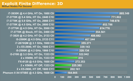
In three dimensions, the E5-2690s still have the advantage, at 7.7% with HT enabled. With HT disabled, the dual X5690 system performs 11.4% better than the Sandy Bridge-E counterparts. The nature of the 3D simulation tends towards a single CPU system performing much better, however.
Implicit Finite Difference (with the Alternating Direction Implicit method)
The implicit method takes a different approach to the explicit method – instead of considering one unknown in the new time step to be calculated from known elements in the previous time step, we consider that an old point can influence several new points by way of simultaneous equations. This adds to the complexity of the simulation – the grid of nodes is solved as a series of rows and columns rather than points, reducing the parallel nature of the simulation by a dimension and drastically increasing the memory requirements of each thread. The upside, as noted above, is the less stringent stability rules related to time steps and grid spacing. For this we simulate a 2D grid of 2n nodes in each dimension, using OpenMP in single precision. Again our grid is isotropic with the boundaries acting as sinks.
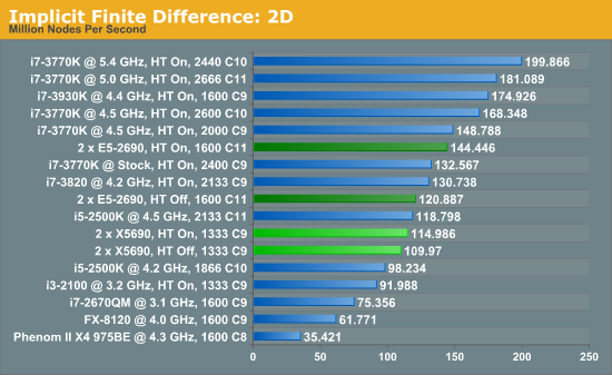
The IPC and increased memory bandwidth of the E5-2690 system comes through here, with the X5690s being 20% slower. The dual CPU nature of the system is still at odds with the coding, as a single i7-3930K at stock should perform similarly.
Brownian Motion
Part of my regular motherboard review testing is to tackle the Brownian motion of particles. This considers one of two physical scenarios - either gas in a vacuum or a dissolved substance in a fluid, where those particles that are free to move can do so. These particles can collide with the medium they are in, each other or the boundaries – in general the system can bypass all these by using the diffusion coefficient (average speed of a particle in a medium). However, the simulation should be probing at least one of them – with the first two situations requiring greater computational complexity than dealing with interactions on a surface.
The movement of these particles is the main computational element of this type of simulation – dealing with either free motion (mean free path in a random direction) or directed motion (applied force on top of free motion). Motion should start with a method to calculate which direction the particle is to travel in, and then any applied force simulated on top – the initial method is at the whim of random number generators and the choice of algorithm. In my original article I go through several methods of generating random motion described in the literature, as well as choosing an appropriate random number generator (too many published methods use basic C++ generators that repeat themselves after a few thousand calls). For simulating, we have various methods:
- If the simulation has a fixed number of time steps, calculate the random numbers before the simulation and use memory calls in the movement algorithm
- Calculate the random numbers on the fly during the algorithm if the time steps for each particle can vary (i.e. no need to track a particle after it collides with a surface)
In our Brownian motion benchmark (3D Particle Movement), we test the six different algorithms used in the literature for random direction movement in both single thread and multithreaded mode. The simulation generates a number of particles, each with its own thread. The thread iterates the particle through a fixed number of steps, and discards the particle. When all the threads have finished, the simulation checks the time to see if 10 seconds have passed - if the 10 seconds are not up, it goes through another loop. Results are then expressed in the form of million particle movements per second for each algorithm, and the total score is the sum of all the algorithms.
This benchmark is wholly memory independent – by generating random numbers on the fly, each thread can keep the position of the particle and the random number values in local cache.
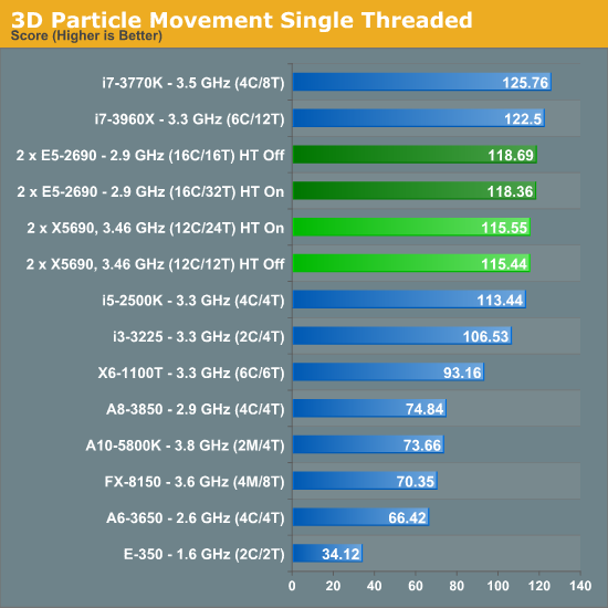
The difference in architectures is most plain to see in our single thread test – both the X5690 and E5-2690 will be applying maximum turbo (3.73 GHz and 3.8 GHz respectively) to similar clocks, meaning the IPC improvements of Sandy Bridge-E give it a 2.5% increase overall despite a mild (1.8%) clock increase.
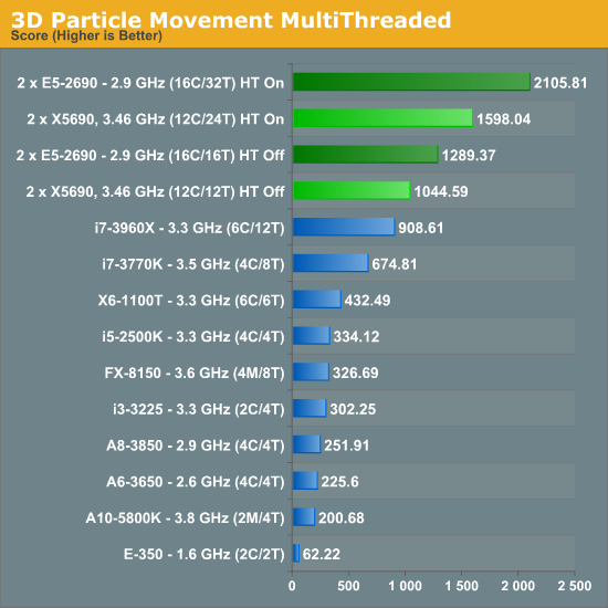
The advantages of more cores for this sort of simulation are plain to see, with the E5-2690 (despite a clock speed difference at full load of 2.9 GHz compared to 3.46 GHz) giving a 32% better result than the X5690.
n-Body Simulation
When a series of heavy mass elements are in space, they interact with each other through the force of gravity. Thus when a star cluster forms, the interaction of every large mass with every other large mass defines the speed at which these elements approach each other. When dealing with millions and billions of stars on such a large scale, the movement of each of these stars can be simulated through the physical theorems that describe the interactions.
n-Body simulation is a large field of calculation with many different computational methods optimized for speed, memory usage or bus transfer – this is on top of the different algorithms that can be used to represent such a scenario. Typically one might expect the running time of a simulation be O(n^2) as each particle in the simulation has to interact gravitationally with every other particle, but some computational methods can be used to reduce this as the effect of gravity is inversely proportional to the square of the distance, and thus only the localized area needs to be known. Other complex solutions deal with general relativity. I am neither an expert in gravity simulations or relativity, but the solution used today is the full O(n^2) solution.
Part of the available code online for C++ AMP revolves around n-body simulations, as the basis of an n-body simulation maps nicely to parallel processors such as multi-CPU platforms and GPUs. For this review, I was able to strip out the code from the n-body example provided and run some numbers. Many thanks to Boby George and Jonathan Emmett from Microsoft for their help.
The code provided detects whether the processor is SSE2 or SSE4 capable, and implements the relative code. We run a simulation of 10240 particles of equal mass - the output for this code is in terms of GFLOPs, and the result recorded was the peak GFLOPs value.
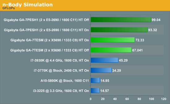
As the n-body example deals with GFLOPs as a result, the numbers were only ever going to be in favor of the E5-2690s, with a 37% increase over the X5690s. Core count, IPC and memory speed play a role with large O(n2) simulations like these. Oddly enough, while HT Off was preferable on the E5-2690s, HT On gives a better result for X5690s.
For completeness, we run our normal motherboard benchmarks.
WinRAR x64 3.93 - link
With 64-bit WinRAR, we compress the set of files used in the USB speed tests. WinRAR x64 3.93 attempts to use multithreading when possible, and provides as a good test for when a system has variable threaded load. If a system has multiple speeds to invoke at different loading, the switching between those speeds will determine how well the system will do.
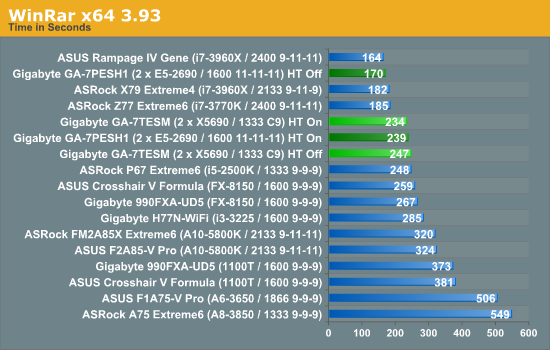
Despite the slight memory difference between the two platforms, using E5-2690s with HT off has a significant 29% advantage over HT being on or the X5690 results.
FastStone Image Viewer 4.2 - link
FastStone Image Viewer is a free piece of software I have been using for quite a few years now. It allows quick viewing of flat images, as well as resizing, changing color depth, adding simple text or simple filters. It also has a bulk image conversion tool, which we use here. The software currently operates only in single-thread mode, which should change in later versions of the software. For this test, we convert a series of 170 files, of various resolutions, dimensions and types (of a total size of 163MB), all to the .gif format of 640x480 dimensions.
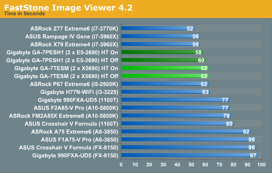
With the single thread speeds being similar, the only separation between our systems should be IPC – and thus as expected the Sandy Bridge-EP system is ahead, but only by 3-6%.
Xilisoft Video Converter
With XVC, users can convert any type of normal video to any compatible format for smartphones, tablets and other devices. By default, it uses all available threads on the system, and in the presence of appropriate graphics cards, can utilize CUDA for NVIDIA GPUs as well as AMD APP for AMD GPUs. For this test, we use a set of 32 HD videos, each lasting 30 seconds, and convert them from 1080p to an iPod H.264 video format using just the CPU. The time taken to convert these videos gives us our result.
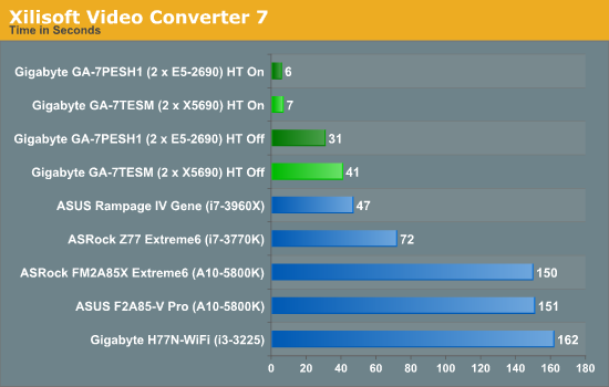
With XVC having many threads is what counts, meaning that 24 threads on a full X5690 system will equal our small video conversion test. At this level, we would need more content to see significant difference. With HT off however, the Westmere-EP result is nearer that of a single 3960X than the E5-2690s.
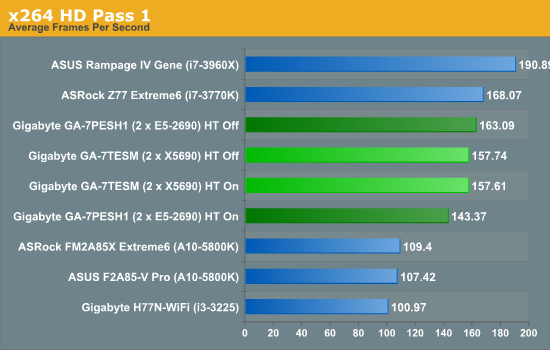
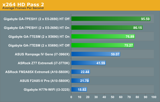
x264 HD Benchmark
The x264 HD Benchmark uses a common HD encoding tool to process an HD MPEG2 source at 1280x720 at 3963 Kbps. This test represents a standardized result which can be compared across other reviews, and is dependant on both CPU power and memory speed. The benchmark performs a 2-pass encode, and the results shown are the average of each pass performed four times.
Is Sandy Bridge-EP an Upgrade Path?
At the beginning of this review, I referred back to Johan’s article on the behind the scenes benefits that Sandy Bridge-EP offers over Westmere-EP, and condensed them into a list for what a non-CS student in a scientific field might have to consider:
- The improved core and µop cache on Sandy Bridge-EP should boost IPC through the roof with calculations that can take advantage, especially advanced trigonometric functions.
- The increase in L3 cache would reduce stress on jumps out to main memory for values, although the improved memory bandwidth would also help in this regard.
- More cores are always welcome – Turbo 2.0 would help with pre-release code testing, which often occurs in debug / single thread mode.
- An increase of memory limits would help various simulation scenarios, as well as aid having VMs of different environments.
- The move up to PCIe 3.0 helps any GPGPU simulation that requires lots of memory transfers back and forth across the bus (matrix solving), as long as the GPU supports PCIe 3.0 (K10, K20X, FirePro, not Xeon Phi which uses PCIe 2.0).
Every scenario that an individual faces, either in the office, the laboratory, or generic work place #147 is going to be different – perhaps only slightly, but different nonetheless. We have to weigh up the pros and cons of the specific workload and make relative suggestions.
For the most part, any simulation which has large parts that can be computed in parallel should be looking at GPUs, unless the thread are ‘dense’ (require lots of memory registers for the serial calculation) or are already optimized for SSE4/AVX. Double precision can also be a hurdle to GPU computing, but the NVIDIA GTX Titan makes the cost a lot more palatable on research grants. Lots of researchers will be dealing with Fortran code tens of thousands of lines long and 20 years old, meaning that porting to GPUs is not a reasonable situation (unless you encourage the research supervisor to apply for a 3 year grant to convert the code). In these cases, make a note of how much memory the simulation needs – if it is sub 2.5 MB, then load up on as many cores as you can get as you will still be in L3 cache on the 20MB L3 processors. For more than that, you will be dealing with memory accesses out to main memory, and unless you are comfortable dealing with NUMA based code and tools (which your Fortran probably is not geared for), then a single fast processor is probably the best bet. MPI based Fortran is where dual processors systems would be best, or for simulations that require more memory than what a single processor can have equipped.
In terms of Westmere-EP vs. Sandy Bridge-EP for our benchmark suite, the relative numbers are:
| Dual E5-2690 vs. Dual X5690 | |||
| Price | +25% (before tax and additional seller markup) | ||
| HT On | HT Off | Recommended Setup | |
| 2D Explicit FD | +12.7% | +7.3% |
GPU or Single Multicore CPU w/High Speed Memory |
| 3D Explicit FD | +7.7% | -10.3% |
GPU or Single Multicore CPU w/High Speed Memory |
| 2D Implicit | +25.6% | +9.9% |
Single CPU High Mem Bandwidth |
|
Brownian Motion Single Thread |
+2.4% | +2.8% | High Single CPU Speed |
|
Brownian Motion Multi Thread |
+31.8% | +23.4% | GPU |
| n-Body | +29.0% | +47.7% | GPU |
| WinRar | +27.4% | +3.4% | High Mem Bandwidth |
| FastStone | +6.5% | +3.2% | High Single CPU Speed |
| Xilisoft Video | +14.3% | +24.4% |
GPU or Multi-CPU |
| x264 Pass 1 | -9.0% | +3.4% | Single CPU |
| x264 Pass 2 | +27% | +24.3% | Multi-CPU |
While we do not get a price equivalent speed up across the board, certain scenarios (Xilisoft, x264 Pass 2) benefit greatly from a dual processor Sandy Bridge-EP system over either Westmere-EP or GPU. Sometimes a GPU is not available, putting the Brownian Motion benchmark through the roof when it comes to more cores. A limiting factor in many of these benchmarks is memory speed – if you do not need a Xeon, then the latest Intel/AMD processors can handle 2133+ MHz memory which provides an absolute tangible boost in finite difference simulation and WinRar.
If we come back to the original question ‘Is moving from Westmere-EP to Sandy Bridge-EP a reasonable upgrade’, in the majority of our scenarios it probably is not – either other alternatives exist that perform better (single CPU, GPU, memory bandwidth) or the price difference is not worth the jump. Remember that most scenarios will have to absorb the whole cost, rather than the cost of an upgrade, and calculating that into the cost/benefit analysis is a major part of the equation. But none of our scenarios need more than 96 GB of memory, PCIe 3.0, VMs for different environments, or use advanced processor instruction sets, which could be vital to your work.
Ivy Bridge-EP is slated for the end of the year, meaning that those on Westmere-EP would probably consider waiting to see what comes out from Intel. If you need a DP system now, then Sandy Bridge-EP is an obvious choice if you want to go down the Intel route, though NUMA related code may benefit from a quad AMD system better. If we get one in for another comparison point, we will let you know.
A final note to give thanks to the Gigabyte server team for loaning us the CPUs and motherboard to make this testing possible.


